| home Java Script MS Access Perl HTML Delphi C ++ Visual Basic Java CGIPerl MS Excel Front Page 98 Windows 98 Ms Word Builder PHP Assembler Link to us Links |
Gathering Data for Simple Calculations with Excel 97
What you will learn from this lesson
With Excel 97 you will:
What you should do before you start this lesson
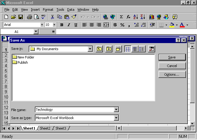
Creating a worksheet with Excel 97 is easy. To help you experience the power of Excel 97, you will use excerpted material from Getting America’s Students Ready for the 21st Century: Meeting the Technology Literacy Challenge, atechnology report from the U.S. Department of Education.
Getting ready to create a worksheet
Exploring the lesson
Excel 97 makes it easy to enhance lessons and reports with data that you and your students can enter and edit quickly. You can create informational charts, grade books with calculating features, data-based statistical programs, graphics, and simple task charts using Excel 97.
Starting new workbooks
Excel 97 makes it easy to design a new workbook to suit your purpose.
Creating a new worksheet

Entering and formatting titles
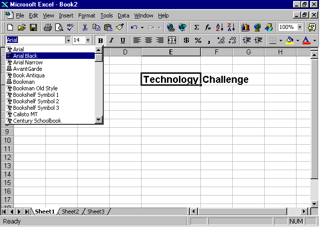
Using titles on the worksheets makes it easier to read and understand the information shown. You can retain the existing styles, create your own styles, or customize your own workbook template. The next exercise illustrates how easy it is to enter and modify font styles and sizes in your worksheet.
Entering and formatting a title on the worksheet
Entering column headings and adjusting widths
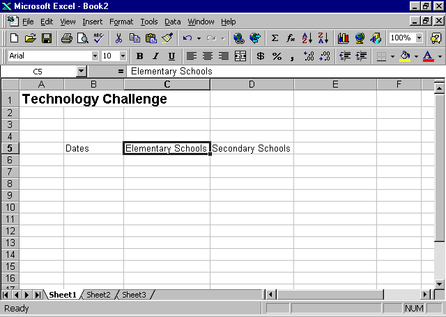
Column headings help you and others understand the data or information you have entered on your worksheet. Sometimes the column heading is too large to fit into a column. Even though it does not show the entire title or formula, the cell still contains everything you entered into it. This exercise shows you how to increase or decrease the column width to fit the information you are entering.
Entering column headings and adjusting their widths
With these easy steps you can customize a template or design your own workbook to present your information.
Arranging text with the Copy, Paste, and Cut commands
With Excel 97, it is easy to modify data. When you and your students use the features in Excel 97 to create a table, you may decide on a different order of column heads or you may want to revise them. It is important to make changes before you build a formula for the chart in order to maintain correct calculations.
Using the Cut, Paste, and Copy commands to arrange text
Entering data
Using Excel 97 is a powerful way to enter and display data or text. For example, you can have Excel 97 display a date showing the month, day, and year with the time, or showing only the first letter of the month, followed by a two-digit year. Numbers can be displayed as whole numbers, numbers with decimals, or numbers written in scientific notation.
Entering data for growth of World Wide Web sites in U.S. schools
|
Dates |
Elementary |
Secondary |
|
1/1/95 |
85 |
110 |
|
4/1/95 |
160 |
360 |
|
7/1/95 |
225 |
380 |
|
10/1/95 |
250 |
660 |
|
1/1/96 |
425 |
900 |
|
4/1/96 |
800 |
1400 |
|
6/1/96 |
1100 |
1720 |
Doing simple calculations
Using Excel 97, you can perform a wide range of mathematical calculations and functions according to what you need from your data. To calculate sums (totals) and percentages, use the mathematical operation of adding numbers to get a total, and then divide each number that was just added by that total.
Calculating the sum of schools with Web sites
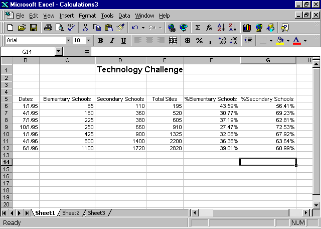
Calculating the percentage of schools with Web sites by category
How you can use what you learned
Microsoft Excel 97 can be used to record and calculate grades. You can create a master record to track student names and assignments. With the student names in a column, and the assignments in a row, you can see at a glance the status of the homework.
You can create your budget and track expenses for school projects. Excel 97 creates many types of graphs to visually explain numerical data. Charts show complex relationships clearly and simply, making it easier for teachers and students to identify patterns in data. Creating graphs will be explained in detail in a later chapter.
Extensions
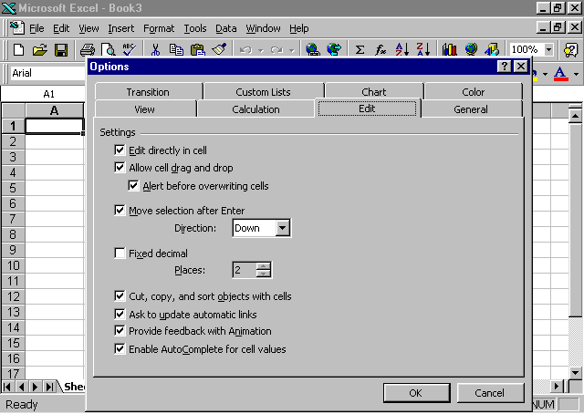
You can change the direction in which the pointer moves when you press enter. If the default direction is to the right, and you are entering data in a column, you can change the default to down. You can change the direction of the pointer to support your movements.
Customizing the enter key
Changing the direction of the enter key
Summarizing what you learned
In this chapter you have explored and practiced: